7. Absorbing boundaries


LAST TIME
Tim Duty described branching processes e.g. birth and death processes:
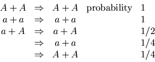
System of n objects of type A.
Elementary processes:

• Death: $A\rightarrow 0$ rate $\lambda$
• Birth: $A\rightarrow 2A$ rate $\beta$

Discussed methods to calculate survival probability and cascade size distribution.


State with no A- particles absorbing state. Once in such a state system trapped and there is no escape!
Today want to discuss how to treat absorbing states in continuum limit.

LIMBO STATE and FICTITIOUS STATE


Master equation for one step processes:

$$\frac{\partial P(n,t)}{\partial t}=(E-1)d(n)P(n,t)-(E^{-1}-1)b(n)P(n,t)$$

If b(0)=0, call n=0 limbo state.
P*(t)=probability of limbo state.
If $b(n)\Rightarrow 0$ as $n \Rightarrow 0$ natural boundary.
Otherwise n=0 artificial boundary.


In continuum limit must avoid treating n=0 as separate case.
If boundary artificial introduce fictitious state n=0. Boundary condition P(0,t)=0.
Normalization:

$$P^*(t)+\sum_{n=0}^\infty P(n,t)=1$$

If $b\propto n$ and $P(n,t)\Rightarrow const.$ as $n \Rightarrow 0$ there is probability current into limbo state!

Example: DIFFUSION NEAR A CLIFF


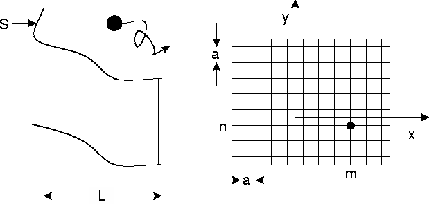
Jumps at rate $\lambda$ distance a in $\pm x$ and $\pm y$ directions.
S absorbing boundary. Master equation:

$$\frac{\partial P(n,m,t)}{\partial t}=\lambda [E_x+E_x^{-1}+E_y+E_y^{-1}-4]P(n,m,t)$$

$$x=na;\;\;y=ma$$

a "smallness parameter"
L= macroscopic length scale
$\Omega=L/a$ system size parameter
S= artificial boundary!

$$\frac{1}{a^2}\Pi(x,y,t)dx dy=P(n,m,t)$$

$$E_x-1=a\frac{\partial}{\partial x}+a^2\frac{\partial^2}{\partial x^2} +\cdots$$

$$E_y-1=a\frac{\partial}{\partial y}+a^2\frac{\partial^2}{\partial y^2} +\cdots$$

Diffusion equation:

$$\frac{\partial\Pi(x,y,t)}{\partial t}=D\left[\frac{\partial^2}{\partial x^2}+ \frac{\partial^2}{\partial y^2}\right]\Pi$$

where $D=\lambda a^2$
Boundary condition $\Pi=0$ on $S \Rightarrow$ eigenvalue problem:




Example:
Square with corners at (0,0),(0,L),(L,L),(L,0) and absorbing sides

$$\Pi(x,y,t)=\sum_{n,m=1}^\infty \alpha_{nm}\psi_{nm}\exp (-\lambda_{nm}t)$$

$$\psi_{nm}=\frac{2}{L}\sin\frac{n\pi}{L}\sin\frac{m\pi}{L}$$

$$\lambda_{nm}=\frac{D(n^2+m^2)\pi^2}{L^2}$$

$$\alpha_{nm}=\int_0^Ldx\int_0^Ldy\psi_{nm}(x,y)\Pi(x,y,0)$$

For long times smallest eigenvalue (ground state) dominates!

$$\lambda_{11}=\frac{2D\pi^2}{L^2}$$

Asymptotic formula for survival probability

$$\Pi_s(t)\approx\frac{8L\alpha_{11}}{\pi^2}\exp(-\frac{2D\pi^2 t}{L^2})$$

Example of problem with natural boundaries:
GENETIC DRIFT
A gene is expressed as allele a or A.
The allele is neutral: there is no competititve advantage to being either A or a.
Stable population size: Population pairs off.
Each pair produces two offspring.

$$\begin{array}{cccll} A+A&\Rightarrow&A+A&{\rm probability}&1... ...&\Rightarrow&a+a&&1/4\\ &\Rightarrow&A+A&&1/4\\ \end{array}$$

Only last two processes change composition of population. Rate of
contributing processes:

$$\beta n(\Omega-n)/\Omega$$

$\Omega =$ size of population.
n = number of individuals of type a.


Master equation:

$$\frac{\partial P(n,t)}{\partial t}=(E_n+E_n^{-1}-2)\frac{\beta n(\Omega-n)}{\Omega}P(n,t)$$

Macroscopic variables $x=\frac{n}{\Omega};\;\tau=\frac{t}{\Omega}.$

$$\frac{1}{\Omega}\Pi(x,\tau)=P(n,t)$$

Fokker-Planck equation



Initial condition $\Pi(x,0)=\Pi_0(x)$.
Try solution on form

$$\Pi(x,\tau)=\sum_{m=0}^\infty \alpha_me^{-\lambda_m\tau}\psi_m(x)$$

$$-\lambda_m \psi_m(x)=\beta\frac{d^2}{d x^2}x(1-x)\psi_m(x)$$

Differential equation singular at x=0,x=1! Cannot impose arbitrary boundary condition.

Require that eigenfunctions well behaved at
x=0,x=1. Try

$$\psi=\sum_{l=0}a_kx^k$$

Get

$$a_{k+1}=\left(1-\frac{\lambda}{\beta(k+2)(k+1)}\right)a_k$$

Radius of convergence of power series x=1. For solution to be well behaved at x=1 require that series breaks off! Eigenvalues:

$$\lambda_m=\beta (m+2)(m+1);\;\;m=0,1,2\cdots$$

Lowest eigenvalue $\lambda_0=2\beta$. Asymptotically, probability that both alleles can be found in population decays as

$$P_s\propto \exp(-2\beta\tau)=\exp(-\frac{2\beta t}{\Omega})$$

Note that lifetime $\propto \Omega$, population size!
Equation for $\psi$ special case of hypergeometric equation. General solution can be expressed in terms of Gegenbauer polynomials! For details see Kimura [1955]

KRAMERS ESCAPE RATE
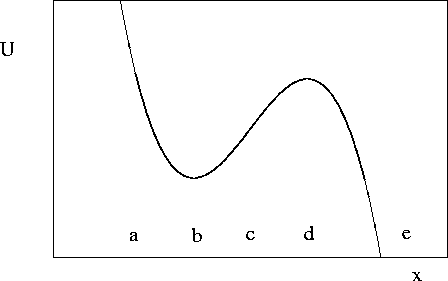
Consider an overdamped partice moving in a potential well near a "cliff".

Force

$$f(x)=-\frac{dU(x)}{dx}$$

• Assume $\Delta U=U(d)-U(b)>>kT$
  Metastable state "quasi-stationary"
  $\Rightarrow J$ approximately independent of x.
  
• Assume particle reaching C are "lost".
  Impose absorbing boundary conditions at e.

Fokker-Planck equation

$$\frac{\partial P(x,t)}{\partial t}= -\frac{D}{kT}\frac{\partial}{\partial x}f(x) P(x,t)+D\frac{\partial^2P(x,t)}{\partial x^2}$$

Probability current

$$J=\frac{D}{kT}f(x) P(x,t) -D\frac{\partial P(x,t)}{\partial x}$$

$$=-D\exp(-\frac{U(x)}{kT})\frac{\partial}{\partial x}\exp(\frac{U(x)}{kT})P(x,t)$$

Integrate from b to e with P(e,t)=0

$$D\exp(\frac{U(b)}{kT})P(b,t)=J\int_{b}^{e}dx\exp(\frac{U(x)}{kT})$$

Assume that near b

$$P(x,t)\approx P(b,t)\exp(-\frac{U(x)-U(b)}{kT})$$

Probability that particle is "near" b

$$p=P(b,t)\exp(\frac{U(b)}{kT})\int_a^c\exp(-\frac{U(x)}{kT})$$

Escape rate



The integrals in the boxed expression above can be evaluated numerically to arbitrary accuracy. In order to get a simple and easy to remember expression we note that the dominant contribution from first integral comes from near minimum. Expand near b

$$U(x)\approx U(b)+\frac{1}{2}kT(x-b)^2\alpha$$

Second integral dominated by contribution from near maximum

$$U(y)\approx U(b)-\frac{1}{2}kT (y-d)^2\beta$$

Get Kramers' escape rate



This is an asymptotic formula valid in the limit $\Delta U/kT\Rightarrow \infty$. See the book of Risken for low order correction terms!

SUMMARY

• Discussed absorbing boundary conditions for
  • artificial boundaries
  • natural boundaries.
• Discussed diffusion near a "cliff".
• Solved a genetic drift problem.
• Derived Kramers formula for escape rate from metastable state

Click here for Return to title page
Click here for 8. Transformations and blow torches