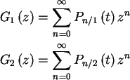


Next: About this document ...
A Simple Branching Process
The model.
Consider a system of A-particles or individuals subject to the
Poisson-distributed random events
![\begin{align*}\text{Death} & :\text{ }
\begin{array}[c]{ll}
A\rightarrow0\ \ \...
...gin{array}[c]{ll}
A\rightarrow2A & \text{rate }\beta
\end{array}
\end{align*}](img1.gif)
The state of zero individuals is an absorbing state. If the system hits this
state it stays there.
The corresponding master equation is
 |
(1) |
Suppose we start with one individual at  .
We'd like to know something
about the sizes and durations of the resulting cascades.
Interesting quantities.
1. Survival probability.
or the number of cascades lasting longer than time t, and in particular, its
asymptotic value
2. Cumulative size distribution
 ,
the number of
cascades larger than size s, or the probability that a cascade involves at
least s individuals.
One finds critical behaviour when
 ,
i.e. all of these quantities behave as power laws

Survival probability.
The survival probability can be found by using the generating function
 |
(2) |
From the generating function, we can find the moments by taking derivative
w.r.t z and then setting z=1.
For example:
and
often the moments
 |
(3) |
are refered to as `factorial' moments.
From the factorial moments, one can alway get back the probabilities
We can use eqn (1) to obtain an equation for the generating function
for this birth-death process. By multiplying by zn and summing over n,
one finds
 |
(4) |
This can be solved using the method of characteristics.
The method of characteristics.
Let
![$\left[ z\left( \tau\right) ,t\left( \tau\right) \right] $](img15.gif) be some
curve in the
be some
curve in the
 plane. The change in G along this curve
is
 |
(5) |
We want to choose a curve such that
Eqn. (4) implies
 is constant along
this characteristic. Integrating
we find
where C is some constant of the curve
 .
Then
 must be some function of C.If we consider initial conditions
such that at t=0, the number of individuals was exactly m, or
 ,
we have
One finds the solution
![\begin{displaymath}G\left( z,t\right) =\left[ \frac{e^{\left( \lambda-\beta\righ...
...\beta z-\lambda\right) +\beta\left( 1-z\right)
}\right] ^{m}
\end{displaymath}](img25.gif) |
(6) |
This complicated looking expression tells us everything we need to know about
this birth death process. Expanding in a power series, we can find
 .
The survival probability is
For
 ,
,
the population becomes extinct. For


For the critical case,
 one finds
 |
(7) |
Exercise. The result for the critical
point can also be found by
solving the (factorial) moment equations. Using eqn. (3) show
that
and that for 1-initial particle b.c , these equations can be recursively
integrated to find
Digression:
An easier method
There's actually an easier way to get the duration results. For this method,
we need conditional probabilities.

For Markov processes, one finds Kolmogorov's forward and backward equations.
Forward equation.
or with
t=t2-t1,
Backward equation.
or with
t=t2-t1,
Note that we can obtain the master equation by multiplying the both
sides of the forward equation by Pm and summing over m, so that one
only need worry about state probabilities at time t2 and not conditional probabilities.
For this simple branching process, the backward equation for 1-initial
individual boundary conditions is
Using the generating functions

the backward equation becomes
but since
subject to the initial condition
hence
Size distribution.
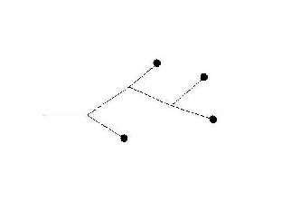
In order to find the size distribution, we look at a generic tree.
The probability of a tree with n leaves is
![\begin{align*}P_{n} & =\left(
\begin{array}[c]{c}
\text{\char93 of trees}\\
...
...ight) ^{2}
}\right] ^{n}\left( \frac{\lambda+\beta}{\beta}\right)
\end{align*}](img49.gif)
Using Stirling's formula
or
with the characteristic size
So the cumulative size distribution
Exercise. Suppose you didn't know Cayley's formula. You can still
calculate the size distribution by using a slightly modified model.
where R is a `removed' individual.
Using a two species generating function
One can use either the backward or forward equation and the relevant method
above to solve for the
 probabilities.
Click here for Return to title page
Click here for 7. Absorbing boundaries


Next: About this document ...
Birger Bergersen
1998-10-03
![]() ,
i.e. all of these quantities behave as power laws
,
i.e. all of these quantities behave as power laws


![\begin{displaymath}G\left( z,t\right) =\left[ \frac{e^{\left( \lambda-\beta\righ...
...\beta z-\lambda\right) +\beta\left( 1-z\right)
}\right] ^{m}
\end{displaymath}](img25.gif)


![\begin{align*}P_{n} & =\left(
\begin{array}[c]{c}
\text{\char93 of trees}\\
...
...ight) ^{2}
}\right] ^{n}\left( \frac{\lambda+\beta}{\beta}\right)
\end{align*}](img49.gif)
![\begin{displaymath}P_{n}\simeq\frac{1}{2\sqrt{\pi}}n^{-3/2}\left[ \frac{4\lambda...
...^{2}}\right] ^{n}\left( \frac{\lambda+\beta}{2\beta
}\right)
\end{displaymath}](img50.gif)


