2. System size expansion


LAST TIME:
Introduced the master equation
for discrete system:

$$\frac{\partial P(n,t)}{\partial t}=\sum_{n'}[W(n\vert n')P(n',t)-W(n'\vert n)P(n,t)]$$

For birth and death processes

$$W(n\vert n')=d(n')\delta_{n,n'-1}+b(n')\delta_{n,n'+1}$$

d=death rate.
b=birth rate.
Macroscopic rate equation

$$\frac{dn}{dt}=b(n )-d(n )$$

Today: Want to study validity of rate equation and fluctuations of n for large system.

EXPANSION OF THE MASTER EQUATION
Expect for large systems:
Mean $\langle n\rangle \propto \Omega =$ system size parameter.
Fluctuations $= n-\langle n\rangle\propto \sqrt{\Omega}$.
Describe this situation as

$$n=\Omega\phi(t)+\sqrt{\Omega} x$$

$\phi(t)=$ non-fluctuating variable.
$\phi(t)$ will satisfy ordinary differential equation (normally just rate equation).

x fluctuating continuous variable with probability distribution $\Pi(x,t)$.

TRANSFORMATION OF VARIABLES

$$n=\Omega\phi(t)+\sqrt{\Omega} x$$

When n fluctuates by an amount $\Delta n$, x will fluctuate by $\Delta x=\Delta n/\sqrt{\Omega}$.

$$P(n,t)\Delta n=\Pi(x,t)\Delta x$$

$$\Pi(x,t)=\sqrt{\Omega}P(\Omega\phi(t)+\sqrt{\Omega} x,t)$$

$$\frac{\partial\Pi}{\partial x}=\Omega\frac{\partial P}{\partial n}$$

$$\frac{\partial P}{\partial t}=\frac{1}{\sqrt{\Omega}}\frac{\p... ...i}{\partial t}- \frac{d\phi}{dt}\frac{\partial\Pi}{\partial x}$$

RAISING AND LOWERING OPERATORS

Ef(n)=f(n+1)

E^-1f(n)=f(n-1)

Master equation

$$\frac{\partial P(n,t)}{\partial t}=\{(E-1)d(n)+(E^{-1}-1)b(n)\}P(n,t)$$

$$E-1=\frac{1}{\sqrt{\Omega}}\frac{\partial}{\partial x}+\frac{1}{2\Omega} \frac{\partial^2}{\partial x^2}+\cdots$$

$$E^{-1}-1=-\frac{1}{\sqrt{\Omega}}\frac{\partial}{\partial x}+\frac{1}{2\Omega} \frac{\partial^2}{\partial x^2}+\cdots$$

Need to substitute into master equation and convert to equation for $\Pi$, sorting terms according to order in $\Omega$. UGH! Example: MALTHUS-VERHULST PROBLEM
Birth and death problem in which a logistic term to takes into account competition. $\Omega$ is the system size parameter.
Birthrate: $b(n)=\beta n$
Death rate: $d(n)=\alpha n +\frac{1}{\Omega}n(n-1)$ The Macroscopic rate equation is




The steady state solutions are
n=0 , and $n=\Omega/(\beta-\alpha)=n_0$
For $\alpha>\beta$, n=0 solution is stable,
n=n₀ is unphysical. (Population dies out.) For $\beta>\alpha,\;\;n=n_0$ stable, n=0 unstable.
Population approaches carrying capacity. Master equation is:



Do our change of variable:

$$\Pi(x,t)=\sqrt{\Omega}P(\Omega\phi(t)+\sqrt{\Omega} x,t)$$

Substitute the expansions for E, E^-1. Find (after some algebra)

$$\frac{\partial\Pi(x,t)}{\partial t}=\Omega^{1/2}\frac{\partial\Pi}{\partial x}[\;] +\{\;\}\Pi+O(\Omega^{-1/2})$$

where

$$[\;]=\frac{d\phi}{dt}+(\alpha-\beta)\phi+\phi^2$$

$$\{\;\}\Pi=(\alpha-\beta+2\phi)\frac{\partial}{\partial x}x\Pi... ...}{2}(\alpha+\beta+\phi)\phi \frac{\partial^2\Pi}{\partial x^2}$$

For the expansion in powers of $\Omega$ to work must have $[\;]=0$. $[\;]=0$ gives

$$\frac{d\phi}{dt}=(\beta-\alpha)\phi-\phi^2$$

Equivalent to macroscopic rate equation!
(Remember $\phi\approx n/\Omega$.)
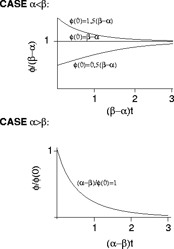
Solution



Solution depends only on net birth rate $\beta-\alpha$.
For

$$\beta>\alpha,\;\;\phi\Rightarrow (\beta-\alpha)=\phi_s\;\; t\Rightarrow \infty$$

$$\beta<\alpha, \;\;\phi\Rightarrow 0, \;\; t\Rightarrow \infty$$

$$\beta=\alpha\;\;\phi\Rightarrow\frac{\phi(0)}{1+\phi(0)t}$$

Will have to discuss the cases separately!






In general:
Require that terms of order $\sqrt{\Omega}$ vanish. Get for terms independent of $\Omega$
in system size expansion


FOKKER PLANCK EQUATION For Malthus-Verhulst problem:



Substitute $\phi$ from solution to macroscopic equation.
Can find results for mean and variance without solving Fokker Planck equation: Have

$$\int_{-\infty}^{+\infty}\Pi(x,t)dx=1$$

$$\langle x\rangle=\int_{-\infty}^{+\infty}x\Pi(x,t)dx$$

$$\langle x^2\rangle=\int_{-\infty}^{+\infty}x^2\Pi(x,t)dx$$

$$\langle x^2\rangle-\langle x\rangle^2=\sigma^2$$

Integrate by parts



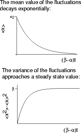
Interested in steady state fluctuations! If $\alpha>\beta$ there is no steady state. Population dies out! $\Omega$ irrelevant! THE CASE $\beta>\alpha$
The population will now approach the macroscopic steady state $\phi_s=\beta-\alpha$

$$\frac{d}{dt}\langle x\rangle=-(\beta-\alpha)\langle x\rangle$$

$$\frac{d}{dt}\langle x^2\rangle=-2(\beta-\alpha)\langle x^2\rangle+ 2\beta(\beta-\alpha)$$

Assuming a (t=0) fluctuation of size x₀ i.e.

$$\langle x(0)\rangle=x_0;\;\langle x(0)^2\rangle -\langle x(0)\rangle^2=0$$

the solution is

$$\langle x(t)\rangle=x_0e^{-(\beta-\alpha)t}$$

$$\langle x(t)^2\rangle -\langle x(t)\rangle^2=\beta(1-e^{-2(\beta-\alpha)t})$$

SUMMARY

• We analyzed a system in terms of a macroscopic variable and fluctuations
  
  $$n=\Omega\phi(t)+\sqrt{\Omega} x$$
  
  

• The master equation was expanded in powers of $\Omega^{-1/2}$.
• Malthus-Verhulst problem used as an example.
• $\phi$ was found to satisfy a macroscopic deterministic rate equation.
• Probability distribution of x satisfied a Fokker-Planck equation.
• The mean and the variance of the fluctuations could be extracted directly from the Fokker-Planck equation.
• While macroscopic equation only depended on effective birth rate
  $\beta-\alpha$, fluctuations contained information about both.

Click here for 3. Fokker-Planck equation Click here for Return to title page