Rolf Luchsinger Oct. 98



10. Molecular Motors



Experimental facts:

• nano-microscale
  ( $\Rightarrow$ thermal noise relevant)
• motors move along linear, periodic structure
  (Kinesin and Dynein on Microtubule)
  (Myosin on Actin)
• energy (ATP) is needed
• two states (bound $\Leftrightarrow$ unbound)
• isothermal ( $\eta_c = 1-T_2/T_1 = 0$)

FORCED THERMAL RACHET
(Magnasco,1993)

LANGEVIN Eq. for an over damped particle



where

f(x) = f(x+l)

$$F_{eff}=\frac{1}{\tau} \int_0^{\tau} F(t) dt = 0$$

$$\langle \xi(t)\xi(t')\rangle =2 k_B T \delta(t-t')$$

Corresponding FOKKER-PLANCK Eq.
(Smoluchoswki equation)

$$\frac{\partial P(x,t)}{\partial t}= \mu \left[-\frac{\partial... ...f(x)+F(t)\Bigg) P+ k_B T \frac{\partial}{\partial x} P \right]$$

with $\mu = 1/\alpha$ (mobility)

Rewrite the Smoluchowski Eq.

$$\frac{\partial P(x,t)}{\partial t}+ \frac{\partial}{\partial x} J(x,t) = 0$$

$$J(x,t) = \mu \left[- k_B T \frac{\partial}{\partial x}P +\Bigg(f(x)+F(t)\Bigg)P\right]$$

Stationary solution:

$$\frac{\partial P(x,t)}{\partial t} = 0\quad \Rightarrow J = const.$$

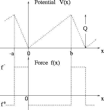
Simplest case: Piecewise linear potential:
$f^- = \;\;\;Q/a$
f⁺ = -Q/b

$$P(x) = \left\{\begin{array}{r@{\; ;\;}l } c_1 \exp(\frac{(F... ...{J}{\mu(F+f^+)} & \;\;\;0 \le x \le b \end{array} \right.$$

1) P(-0) = P(0) (continuous)
2) P(-a) = P(b) (periodic)
3) $\int_{-a}^b P(x) dx = 1$ (normalized)

$$1) \Rightarrow c_1-c_2 = \frac{J}{\mu}\left( \frac{1}{F+f^+}-\frac{1}{F+f^-}\right)$$

$$1) + 2)\quad \Rightarrow \quad \frac{c_1}{c_2} = \frac{\ex... ...rac{F b - Q}{k_B T}) - 1} {\exp(\frac{-F a - Q}{k_B T}) - 1}$$

Investigate different cases:

a.) F = 0:

$$\frac{c_1}{c_2} = \frac{\exp(\frac{- Q}{k_B T}) - 1} {\exp(\frac{- Q}{k_B T}) - 1} = 1 \quad \Rightarrow J = 0$$

b.) $F \ne 0,\;\; a = b \Leftrightarrow V ={\rm sym}$:

$$\frac{c_1}{c_2} = \frac{\exp(\frac{Fa- Q}{k_B T}) - 1} {\exp(\frac{-Fa-Q}{k_B T}) - 1} \ne 1$$

$$\tilde{F} := -F\; \Rightarrow \;\frac{\tilde{c_1}}{\tilde{c_2... ...\; \Rightarrow \;\tilde{c_1} = c_2, \tilde{c_2} = c_1 \quad 3)$$

$$\tilde{c_1}-\tilde{c_2} = \frac{J}{\tilde{J}}(c_1-c_2) \; \Rightarrow \; \tilde{J} = -J$$

$$J_{av} = \frac{1}{\tau}\int_0^{\tau} J(F(t)) dt = \frac{1}{2} (J(F)+J(-F)) = 0$$

c.) $F \ne 0,\;\; a \ne b \Leftrightarrow V ={\rm asym}$:

$$J(F) = \frac{P_2^2 \sinh(lF/2k_B T)}{k_B T (l/Q)^2 \{\cosh[... ...F/2)/k_B T]-\cosh(lF/2k_B T)\} -(l/Q)P_1P_2\sinh(lF/2k_B T)}$$

where $P_1 = \Delta +\frac{l^2-\Delta^2}{4}\frac{F}{Q},\;\; P_2 = \left(1-\frac{\Delta F}{2Q}\right)^2 - \left(\frac{lF} {2Q}\right)^2$
$\;\;\;\quad \quad l = a + b, \;\; \Delta = b-a$


$\quad J(-F) \ne -J(F)\quad \Rightarrow \quad J_{av} \ne 0$

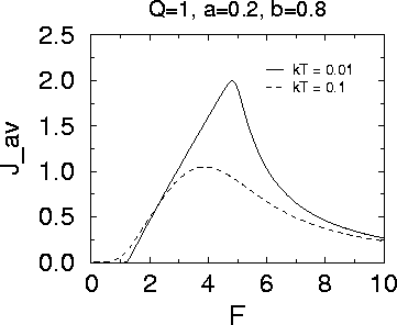
The average probability current J_av as a function of the magnitude of the external forcing.

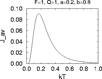
The average probability current J_av as a function of the temperature.





A net probability current J_av results for:

• Asymmetric Potential
• Finite Temperature
• Forcing with time correlations

There are physical applications of the Forced Thermal Ratchet (Molecular Pumps, Filters) but the relevance for biological molecular motors is not clear.

TWO-STATE MODEL
(Prost et al, 1994)


Instead of the time-correlated forcing, this model assumes a two-state system (bound/unbound) for the motor. The external action (ATP hydrolysis) drives the transition rates between the two states away from their equilibrium values.

$$\frac{\partial P_1}{\partial t}+ \frac{\partial}{\partial x} J_1 = -w_1(x)P_1+w_2(x)P_2$$

$$\frac{\partial P_2}{\partial t}+ \frac{\partial}{\partial x} J_2 = w_1(x)P_1-w_2(x)P_2$$

$$J_i = \mu_i \left[- k_B T \frac{\partial}{\partial x}P_i - P_i\frac{\partial}{\partial x} V_i \right]$$

This set of equations can be transformed to an equation for the total probability current J=J₁+J₂ as a function of P=P₁+P₂

$$J = \mu_{eff} \left[- k_B T \frac{\partial}{\partial x}P - P\frac{\partial}{\partial x} V_{eff} \right]$$

$$\mu_{eff} = \mu_1 \lambda +(1-\lambda)\mu_2,\;\;\; \lambda= \frac{P_1}{P}$$

$$V_{eff}(x)-V_{eff}(0) = \int\limits_0^x dx' \frac{\mu_1 \lamb... ...\partial}{\partial x'}V_2}{\mu_1 \lambda + \mu_2 (1-\lambda)}$$

$$\quad \quad \;\; + k_B T \ln (\mu_{eff})\vert _0^x$$

If the effective force
F_eff = (V_eff(x+l)-V_eff(x))/l
vanishes, then J vanishes.


One can show that

• V₁, V₂ symmetric $\Rightarrow F_{eff} = 0$
• $w_1(x) = w_2(x)\exp((V_1(x)-V_2(x))/k_B T)\\ \Rightarrow F_{eff} = 0$ (detailed balance)
• detailed balance broken by energy input
  through ATP $\Rightarrow F_{eff} \ne 0 \Rightarrow J\ne 0$

An effective force can be obtained by breaking detailed balance.

The basic mechanism for the Two-State System can be understood from the Figure. A particle makes a transition from 1 to 2. It diffuses in state 2. After a certain time there is a finite probability that it will fall into the next well during the transition from 2 to 1.

Matching of transition rates, diffusion rate and potential form is important.

SUMMARY

• Basic understanding of molecular motors
  emerges
• Theories based on Fokker-Planck equations
• Three important ingredients:
  -broken symmetry
  -noise
  -correlated forcing/broken detailed balance
• Stochastic resonance behavior
• So far the importance of noise in biological motors not proven, but if models are correct, then:

Noise keeps us going!

REFERENCES:


M.O. Magnasco, Phys.Rev.Lett. 71, 1477 (93)
J. Prost et al, Phys.Rev.Lett. 72, 2652 (94)
F. Jülicher et al, Rev.Mod.Phys. 69, 1269 (97)
R.D. Astumian, Science 276, 917 (97)


Click here for Return to title page
Click here for 11. Lévy-stable distributions