15. Random walk in fractal time. Correlated walks
LAST TIME

• Considered continuum time random walks in which waiting time distribution were Lévy-stable.
• If the waiting distribution had no mean found subdiffusion, i.e. typical excursion grew slower than
  $\sqrt{t}$ for large times.
• Typical situations:
  • Diffusion in lattices with traps.
  • Diffusion in systems with many "blind alleys", e.g. percolation clusters.

TODAY we will discuss:

• Random walks where the number of jumps per unit time is Lévy stable.
• Associated phenomenon intermittency
  • Near laminar flow $\Rightarrow$ turbulence transition typically have bursts of violent activity followed by quiet periods.
  • Similar behavior of fluctuations near first order (discontinuous) phase transitions.
  • In financial markets one observes periods with high volatility and enormous trading volumes interspersed with slow periods.
• We will also start discussing situation were jumps are correlated.

INTERMITTENCY
Toy model for price fluctuations
Consider a market where

• x(t) represents the change in price of a certain commodity over a period of time t.
• where we work with changes in price, rather than price itself, because we don't want to be bothered by having to make prices positive definite.
• Each transaction leads to a small price change with probability ditribution p(x).
• Assume these price changes uncorrelated.
• Probability after n transactions P(x,n).
• n= transaction volume governed by probability distribution $\psi(n,t)$.

Probability distribution for price change x after time t:

$$\Pi(x,t)=\sum_{n=0}^{\infty}P(x,n)\psi(n,t)$$

For simplicity assume Gaussian distribution for the effect of a single transaction:

$$p(x)=\frac{1}{\sqrt{2\pi\sigma^2}}\exp(-\frac{x^2}{2\sigma^2})$$

Without lack of generality we can choose our unit price to be such that $\sigma=1$.

The price change distribution after n transactions is thus

$$P(x,n)=\frac{1}{\sqrt{2\pi n}}\exp(-\frac{x^2}{2n})$$

We finally assume that the distribution for transaction volume is Lévy stable for large t:

$$\psi(n,t)\propto \frac{1}{t^{\alpha +1}}\;\;as\;t\rightarrow\infty$$

As a first example let us assume transaction volume follows Lévy-Smirnov distribution:

$$\psi(n,t)=\frac{bt}{(2\pi)^{1/2}n^{3/2}} \exp(-\frac{b^2t^2}{2n})$$

Choose unit of time so that b=1! Substituting we find

$$\Pi(x,t)=\sum_{n=0}^{\infty}P(x,n)\psi(n,t)$$

$$=\int_0^\infty dn \frac{1}{\sqrt{2\pi n}}\exp(-\frac{x^2}{2n}) \frac{t}{(2\pi)^{1/2}n^{3/2}} \exp(-\frac{t^2}{2n})$$

where we approximate n to be a continuous variable.
A change of variable $n\Rightarrow y=1/n$ yields

$$\Pi(x,t)=\frac{t}{2\pi}\int_0^\infty dy \exp\frac{-y(x^2+t^2)}{2}$$

or

$$\Pi(x,t)=\frac{t}{\pi(x^2+t^2)}$$

Price distribution Cauchy with $\alpha=1$!

In the general case we note from

$$\Pi(x,t)=\sum_{n=0}^{\infty}P(x,n)\psi(n,t)$$

$$=\int_0^\infty dn \frac{1}{\sqrt{2\pi n}}\exp(-\frac{x^2}{2n}) \psi(n,t)$$

that

$$\langle x^2\rangle=\int_{n=0}^\infty n\psi(n,t)$$

We find that

• $\langle x^2\rangle=\infty$ if $\alpha<1$
• $\langle x^2\rangle <\infty$ if $\alpha>1$
• From the central limit theorem we find that the prize will undergo Brownian motion if $\alpha>1$ over a coarse enough time scale.
• Feller[1971] has shown that the distribution $\Pi$ is Lévy stable with exponent $2\alpha$ if $\alpha<1$.

The rôle of "fractal time" distribution of prizes in economics is discussed in detail in Mandelbrot[1997].

We next wish to consider "walks" were successive events are "correlated", i.e. are not indenpendent of each other. In order to lay the groundwork look at one more uncorrelated example:


FREELY JOINTED CHAIN
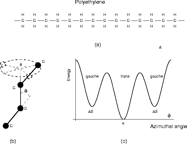
Consider a polymer such as polyethylene which is a chain of molecules

$$-CH_2-CH_2-CH_2-\cdots$$

Our discussion of the polymer problem be largely taken from chapter 8 of Plischke and Bergersen [1994].
Let R_i be the position of the i-th carbon atom and r_i=R_i+1-R_i a vector representing the i-th bond.
We first assume that the chain is freely jointed i.e. each bond points in an arbitrary direction.
The probability that a N+1-carbon chain has an end to end separation R is then

$$P_N(\vec{R})=\Pi_{i=1}^{N}[\frac{1}{4\pi a^2}\int d^3r_i \delta(\vert r_i\vert-a)]$$

$$\times \delta(\vec{R}-\sum_{i=1}^N\vec{r}_i)$$

with a the length of the bond

Fourier transform:

$$F(\vec{k})=\int d^3RP_N(\vec{R})e^{i\vec{k}\cdot\vec{R}}$$

$$=\Pi_{i=1}^N\left(\frac{1}{4\pi a^2}\int d^3r_ie^{i\vec{k}\cdot\vec{r_i}} \delta(\vert\vec{r}_i\vert-a)\right)$$

$$=\left(\frac{\sin(ka)}{ka}\right)^N$$

For large N the function F(k) is sharply peaked at k=0:

$$\ln F(\vec{k})\approx N\ln(1-\frac{k^2a^2}{6})\approx-\frac{Nk^2a^2}{6}$$

and we see that for large N the freely jointed chain is Gaussian

$$P_N(\vec{R})=\int\frac{d^3k}{(2\pi)^3}\exp\left(-\frac{Nk^2a^2}{6} -i\vec{k}\cdot\vec{R}\right)$$

$$=\left(\frac{3}{2\pi Na^2}\right)\exp\left(-\frac{3R^2}{2Na^2}\right)$$

PERSISTENCE LENGTH
Polymers such as polyethylene are not freely jointed. The angle between successive carbon carbon bonds is fairly rigidly fixed at $\theta \approx 68^o$
As our next approximation we put

$$\vec{r}_{i}=\vec{r}_{i+1}\cos\theta-\vec{w}_{i+i}$$

where $\vert\vec{w_i}\vert=a\vert sin\theta\vert$ and $\vec{w}_i\cdot\vec{r}_i=0$. We assume that $\langle \vec{w}_i\rangle=0$

$$\langle \vec{r}_i\cdot\vec{r}_{i+n}\rangle=\langle \vec{r}_{i+1}\cdot\vec{r}_{i+n}\rangle\cos\theta=a^2\cos^n\theta$$

We find for the mean square displacement

$$\langle R_N^2\rangle=Na^2+2\sum_{n>m}\langle\vec{r}_n\vec{r}_m\rangle$$

$$=Na^2+2a^2\sum_{n=2}^{N}\sum_{m=1}^{n-1}\cos\theta^{n-m}$$

After some manipulation of geometric series one finds that the leading term of order N is

$$\langle R_N^2\rangle=Na^2\frac{1+\cos\theta}{1-cos\theta}$$

SHORT VS LONG RANGE CORRELATION
For the freely jointed chain $\langle R_N^2\rangle=Na^2$. We conclude that the correlated random walk is still Gaussian, but with an effective persistence length

$$a_K=\sqrt{\frac{1+\cos\theta}{(1-cos\theta)}}$$

We can make the model more realistic by noting that the orientation of the vector w_i is not uniformly distributed in the plane.





Instead w_i will take into account one of three possible directions (two "gauche" and one "trans"). This will not change the fact that short range correlations will not affect the Gaussian nature of the random walk - it will only modify the value of the persitence length!
This picture changes when the correlations become long range!

THE SELFAVOIDING RANDOM WALK If a polymer is disolved in a good solvent in a dilute solution it will tend to "swell" i.e. occupy a larger volume than it otherwise would. In a "good solvent" the only effective interaction between sections of the polymer is the excluded volume effect - two segments of the polymer cannot occupy the same physical space. In a dilute solution this excluded effect volume only acts on elements of the same chain. The correlations introduced by the restriction of self-avoidance will be long range and cannot be taken into account by introducing a new effective persistence length!


Empirically on finds that the mean square end-to-end distance of selfavoiding walks scales as

$${\bf R}_N^2\propto N^{2\nu}$$

where nu depends on the dimensionality d of the medium in which the medium takes place, but is otherwise believed to universal i.e. independent on the type of lattice, or if the walk is continuous or discrete.


In one dimension we must have $\nu=1$, the only possible self-avoiding walk is one which continues in a straight line.
For $d=2,\; \nu\approx 3/4$ (this value is likely exact), while for $d=3, \; \nu\approx 0.75$. For $d\geq 4,\;\nu=1/2$ which is the same value as we have for the Gaussian random walk. Hence, for $d\geq 4$ self-avoidance is irrelevant. Let us next review a few different approaches to the problem of computing the scaling exponent $\nu$.

COUNTING WALKS
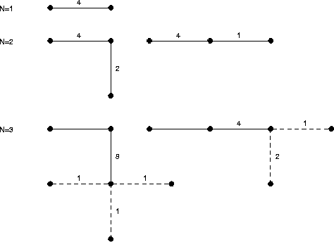
As an example consider the self-avoiding walks on a square lattice. The simplest way to construct all N-step walks is to proceed recursively-that is to add one step in all possible ways to the N-1 step walk. The self-avoiding walks up to order 3 on the square lattice are listed below:





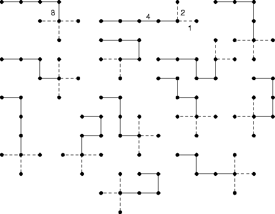
Next, we consider the walks of order 4 and 5:





The average end-to-end distance can then be calculated from

$$S^2_N=\cal{N}^{-1}\sum_{j=1}{\cal{N}} R_N^2(j)$$

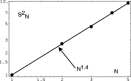
Enumeration gives

$$S^2_1=1,\;S^2_2=frac{8}{3},\; S^2_3=\frac{41}{9},\; S^2_4=\frac{176}{25},\;S^2_5=\frac{679}{71}$$

The results are plotted in a log-log plot below





We find a good fit to $\nu\approx 0.7$. Clearly, more accurate results can be obtained by goind to higher order- which is quite possible with modern computers.

SUMMARY

• In previous lectures we showed that
  • Random walk is non-Gaussian if jump-distribution is Lévy-stable
    with $0<\alpha<2$. superdiffusion.
  • Subdiffusion if waiting time distribution Lévy stable with $0<\alpha<1$.
• Today showed Random walk Lévy -like with $\alpha'=2\alpha$, if transaction rate distribution is Lévy-stable with $0<\alpha<1$
• Began to talk about correlated random walks.
• Showed that if correlations are short range the Gaussian nature of walk prevails, with a different persistence length.
• Started to talk about the self-avoiding random walk.

Return to title page